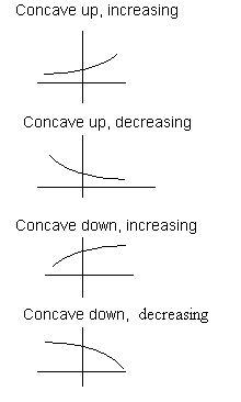
 Four graphs of exponential functions are shown on the right. The graphs depict the four possible behaviors of an exponential function.
When you have finished this lesson:
| Start of Year | Co. A Salary | Co. B Salary |
| (Time) | Linear | Exponential |
| 1 | $40,000 | $40,000 |
| 2 | $42,000 | $42,000 |
| 3 | $44,000 | 44,100 |
| 4 | $46,000 | 46,305 |
| 5 | $48,000 | 48,620 |
| 6 | $50,000 | 51,051 |
Let's now move on to the processing of determining a possible equation for a curve when you are given two points.
Exponential equations: y = abx
- the value of a is equal to the value of the y coordinate of the point.
- use the (x,y) pair of the other point in the formula. The only unknown is b, so solve for it.
- rewrite the equation using the values for a and b that you just found.
Example: put an exponential equation through the points (0, 5) and (3, 40)
- The first point is on the y axis so the y coordinate 5 is equal to a
5 = ab0
b0 = 1 so 5 = a
- use the other point: 40 = 5b3
b3 = 40/5 = 8
- This means that b is the cube root of 8 which is 2
- the formula is y = 5(2)x
- If we want the value of the function when x = 3 it is given by y = 5(2)3 = 5(8) = 40
- take the ratio of the y values for the two points and set it equal to abx using the value of x for each point.
- the a's cancel and you are left with the ratio of the y's (which are numbers) equal to the ratio of b to two different powers. Solve for b.
- rewrite the equation using the value of b you just calculated and the x and y values of one of the points. The only unknown in the equation will be a. Solve for a.
- write the equation of the function y = abx
Example: Put an exponential equation through the points (2, 45) and (4, 405)
- take the ratio of the y values and solve for b (the aĺs cancel)
- 405/45 = b4/b2
- 9 = b2, solving for b; b = + or - 3, but b>0 so only +3 works
- rewrite the equation using your value of b and one of the points, we will use the point (2, 45)
- 45 = a(3)2
- 45 = a (9)
- a = 45/9 = 5
- write the final equation using the values of a and b found above y = 5(3)x
- If we want the value of the function when x = 2 we calculate it as y = 5(3)2 = 5 (9) = 45
Exponential Graphs and Concavity
 Four graphs of exponential functions are shown on the right. The graphs depict the four possible behaviors of an exponential function.
- A graph can be concave up and increasing such as the first figure. In this case the graph bends upwards and the rate of change of the function is increasing (it is getting steeper). Such a function is described as being concave up and increasing.
- The second graph on the right is decreasing at a decreasing rate, meaning it is decreasing but the rate of change is slowing (slope is getting less negative)
- The third graph is concave down and increasing. The graph is increasing but the rate of growth is slowing, the curve is getting less steep (slope is getting less positive)
- The final graph on the right is concave down and decreasing. The graph is decreasing and the rate of decrease is growing, the curve is getting more steep (slope is getting more negative)