Regression

Linear Regression

When analyzing "real world" problems the analyst can be presented with a series of data points that represent data collected during the course of operations. For example a firm may have information on expenditures for advertising and product sales. Similarly a government may have data on population as a function of time. Obviously there are many other possibilities. In some cases what the analyst would like to do is turn the data into a mathematical formula that can be used to predict future results based on the information at hand. One technique for developing a mathematical formula is called Least Squares or Linear Regression. This involves fitting an equation of the form y = mx + b to the data. This section will discuss the process of determining the linear relationship between a y variable (dependent variable) and an x variable (independent variable).

Step 1 - Look at Your Data - Scatter Diagrams

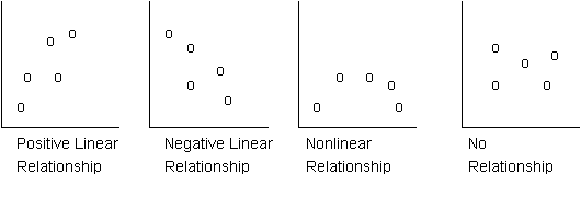
The first step in analyzing data is to plot the data points on an xy grid and look at the data to see if there is a relationship between the points. A Plot of points on an xy grid, without connecting the dots, is called a scatter diagram. The four scatter diagrams shown below demonstrate four possibilities. In the figure on the left there is a positive relationship between x and y and it appears to be reasonably linear. In the next figure there is a negative relationship beteen x and y and it appears to be linear. In the third figure there is clearly a relationship between x and y but it is not linear. Finally, in the last case there does not appear to be any relationship between x and y.

Step 2 - Straight Line Data - Linear Regression

If the scatter diagram of your data looks like a straight line (linear) relationship the next step is to perform a linear regression. The data does not have to perfectly fit a straight line. But it should show that your points tend to follow a straight line trend as in the first two figures shown above.
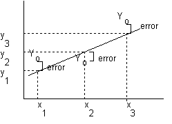
A least square regression provides us with the "best" straight line that can be put through the data. The line is best in the sense that the sum of the squared error from this line is smaller than from any other line that could be drawn. The figure shown below demonstrates the concept. When x took on the values of x₁, x₂, x₃ y was observed to take on the values y_o, y_o stands for the observed value of y when x took on a particular value . The line shown would predict a value of y that is different from that actually observed, thus there is an error. If you calculate those errors and square them (y_line - y_o)² the sum of the squared errors will be smaller for a least squares line than for any other line you could draw. This is what is meant by a best fit line.

Your PC or your calculator should have software that will allow you to quickly calculate the regression line. To illustrate the process let's use some data from history. We will use this data to demonstrate how to calculate the correlation coefficient and also to serve as a cautionary note in that even though we will get a high correlation the predictive value of the relationship is quite questionable for some predictons.
The Lusitania - It is highly probable that you have all heard of the Titanic a very famous ship that sunk after striking an iceberg (in 1912). Fewer of you have probably ever heard of the Lusitania, a ship that sunk after being torpedoed by a German Uboat (in 1915). The Lusitania was also an historic ship. When the Lusitania was being built it was decided to use turbine engines to power the vessel. At the time this was a major change and promised great advantages in terms of speed and efficiency. The estimates of the cost to build the vessel as a function of the vessel's top speed (in knots) is shown in the figure below.

Speed (knots) Cost (pounds sterling)

20 350,000

21 400,000

22 470,000

23 575,000

24 850,000

25 1,000,000

26 1,250,000

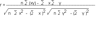
We are going to use the above data to calculate the correlation between ship cost and speed. In doing so we will use cost data in millions as opposed to the way the numbers are shown above. This means that 350,000 will become 0.350 The purpose of this is to simplify the data entry and calculation process, it will not change our final answers. To calculate the correlation coefficient we need:

the sum of the x column and the sum of the y column
on each line multiply x times y and then add the resulting column
square each value of x and y and total the two columns

If you take the above actions you should get the sum of the x column as 161, the sum of the y column as 4.895, the sum of the x² column as 3731, the sum of the y² column as 4.1190 and finally the sum of the x times y column as 116.865. If you use these numbers in the correlation coefficient equation given above you should get a value of r (the correlation coefficient) of 0.9695. As the absolute value of r is very close to 1 this indicates a strong correlation between the two variables. Remember r is between -1 (perfect negative correlation) and +1 (perfect positive correlation), with 0 indicating no correlation.
Our last step will be to use the data to calculate a linear equation (regression equation) that allows us to predict values of cost if we are given values of speed. The general form of our equation is C_p = mS + b Where C_p stands for predicted cost, S stands for speed, m is the slope of our line and b is its y axis intercept. The figure shown below provides the formulas for the necessary calculations.

Using the data given in the table (above) the calculated value of the slope, m, is 0.1529 (rounded to four places) and the value of b is -2.8164 (also rounded to four places). The equation is y = 0.1529x - 2.8164. If we wanted to have a predicted value for a speed of 22.5 knots we would use x=22.5 in the equation: y = 0.1529(25) - 2.8164 = 0.6239 million pounds sterling. As you can see from the data this is somewhat above the actual value of between 0.470 and 0.575 (million pounds sterling). In another section we will fit other functions to this data to see if we can improve the estimates. Note that if we had tried to estimate the cost of a 50 knot ship (not possible at that time) our equation would have given us a number even if it was not possible to build such a vessel at that time. The lesson here is that you need to be careful when you predict outside the domain of values already observed.

Practice Problem 1 - Linear Regression - Using the data in the table shown below calculate the regression coefficient, r and the equation of the regression line y = b_o + b₁x.

x 0 1 2 3

y 1.5 2.5 5.5 6.5

Answer to the practice problem.
All of the values needed to calculate r and the regression equation are calculated in the table shown below.

x y x² y² xy

0.00 1.50 0.00 2.25 0.00

1.00 2.50 1.00 6.25 2.50

2.00 5.5 4.00 30.25 11.00

3 6.5 9.00 42.25 19.50

--- --- --- --- ---

6.00 16.00 14.00 81.00 33.00

Speed (knots)	Cost (pounds sterling)
20	350,000
21	400,000
22	470,000
23	575,000
24	850,000
25	1,000,000
26	1,250,000

x	y	x²	y²	xy
0.00	1.50	0.00	2.25	0.00
1.00	2.50	1.00	6.25	2.50
2.00	5.5	4.00	30.25	11.00
3	6.5	9.00	42.25	19.50
---	---	---	---	---
6.00	16.00	14.00	81.00	33.00