Hypothesis Tests
Hypothesis Tests
The steps in the classical hypothesis test process are as follows:
- Define the null and alternative hypotheses
- Establish the level of significance
- Select the appropriate test statistic
- Use the level of significance and the test statistic to build your decision rule.
- Using the sample data calculate the value of the test statistic.
- Reach a conclusion and fail to reject or reject the null hypothesis
Examples - Large Samples, Single Populations, Test of Mean and Test of Proportion
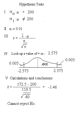 Example 1 - One population, large sample mean
- The null hypothesis is that the mean is equal to 12. The Alternative is that the mean is not equal to 12.
- The level of significance is set at alpha = 0.02
- n>30 so we have a large sample and can use the z distribution.
- Now we need to build a decision rule. We have a two tailed test so there is 0.01 in each tail. Using 0.5000 - 0.01 = 0.4900 we go to table A-2 and find that z is equal to plus and minu 2.33. If we calculate a value of z between -2.33 and +2.33 we will not reject the null hypothesis. If we calculate a value of z that is greater than 2.33 or less than -2.33 we will reject the null hypothesis and accept the alternative hypothesis.
- Using the given data we have z equal to (12.19 - 12)/(0.11/Square root(36)) = 10.36.
- The sample statistic, 10.36, is well past our critical z value of 2.33 so we will reject the null hypothesis and accept the alternative hypothesis.
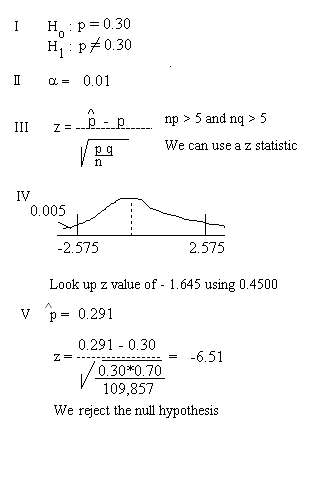 Example 2, One population, proportions
- The null hypothesis is that the population proportion is greater than or equal to 0.10. The alternative is that the population proportion is less than 0.01
- The level of significance is set at alpha = 0.05
- Both np and nq are greater than 5 so we can use the z distribution.
- Now we need to build a decision rule. We have a one tailed test so there is 0.05 in the tail. Using 0.5000 - 0.05 = 0.4500 we go to table A-2 and find that z is equal to 1.645. In this case we have a left-tailed test. Small values of the sample proportion would lead us to reject the null hypothesis. If we calculate a value of z less -1.645 we will reject the null hypothesis and accept the alternative hypothesis. Otherwise we will not reject the null hypothesis.
- Using our data we calculate the value of z as (0.09 - 0.10)/Square Root(0.10 * 0.90/1233) = 1.17.
- The value that we have calculated falls in our do-not-reject the null hyopthesis region.
Examples - Large Samples, Two Populations, Test of Mean - Independent and Dependent Samples
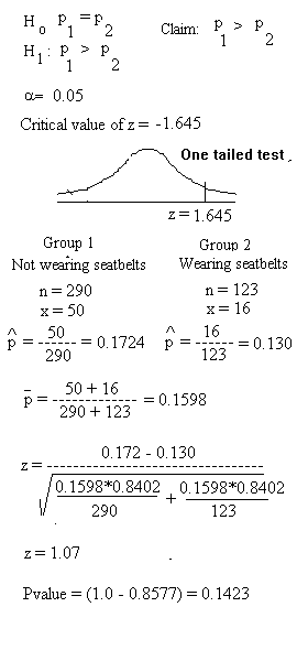 Example 3 - Two populations, large sample, mean
- The null hypothesis is that the mean number of days in ICU for children not wearing a seat belt (Group 2)is less than the mean time spent in ICU for children who were wearing a seat belt (Group 1). The alternative hypothesis is that children not wearing seat belts spent more time in the ICU.
- The level of significance is set at alpha = 0.01 and we have a one-tailed test so all of alpha goes into the left tail.
- n or both groups is >30 so we have a large samples and can use the z distribution.
- Now we need to build a decision rule. We have a one-tailed test so there is 0.01 in the left tail (see figure). Using 0.5000 - 0.01 = 0.4900 we go to table A-2 and find that z is equal to -2.33. If we calculate a value of z that is greater than -2.33 we will not reject the null hypothesis. If we calculate a value of z that is less than -2.33 we will reject the null hypothesis and accept the alternative.
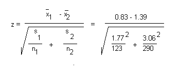 Using the given data, which is repeated in the figure on the left we calculate z as -2.3301. We just barely reject the null hypothesis and accept the alternative. If we calculate the p value we get 0.0099, which is very close to our alpha (0.01).
 Example 1 - One population, large sample mean
 Example 2, One population, proportions
 Example 3 - Two populations, large sample, mean
 Using the given data, which is repeated in the figure on the left we calculate z as -2.3301. We just barely reject the null hypothesis and accept the alternative. If we calculate the p value we get 0.0099, which is very close to our alpha (0.01).