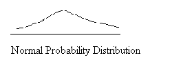
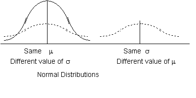
The Concept - When we were dealing with discrete probability distributions each value of x was related to a specific probability. In continuous probability distributions we can't point to specific values of x with spaces between the x values. The values of x all flow together. Thus when we discussed the Empirical Rule we talked about 68% of the data being between the mean plus one standard deviation and the mean minus one standard deviation (mean +s and mean-s). When dealing with with continuous distributions, and in our case it will usually be the normal distribution (pictured below) we will talk about the probability that x will be between certain values.
For continuous distributions the probability that the variable will fall between two values is the area under the curve between those values. In our case one of the values will always be the mean of the probability distribution. To determine a probability we will start with a z Score which is calculated as z = (X - Mean)/Standard Deviation. With the use of a z Score we will be able to transform any normal probability distribution into a "Standard Normal Distribution.".
Why do we need to do this? If you remember our work with the Binomial Distribution you remember that there was a table for every value of n (sample size) with rows (x values) and columns (p values - probabilities) for a range of values of n, x and p. Even though our tables only went to n=15 they were sizeable. If we were to build normal distribution tables for evern conceivable value of the mean and standard deviation we would have a formidable tome! Fortunately there is a better way, and that is transform any normal distribution into the standard normal through use of the z Score. In essesnce we are finding out how many standard deviations a point is from the mean. We will then use the properties of normal distributions to turn that value into a probability.


Standard Normal Distribution - For the standard normal distribution the mean is 0 (zero) and the standard deviation is 1. Let us assume that we have a pressure difference guage that should always read zero when there is no difference in pressure between two containers. Unfortunately no instrument is perfect. Ours has a mean reading of 0 pounds per square inch when pressures are equal and a standard deviation of 1 pound per square inch (psi). So there will be times when our guage will read 0.5 psi even when pressures in the two areas are the same. We would like to be able to determine the probability of our being off by various amounts. What is the likelihood that our guage will read 1 psi when it should read 0 psi? If we calculate the z Score we have z = (1 - 0)/1 = 1. We know from the empirical rule that there is a 68% chance that a value will fall within plus or minus one standard deviation of the mean. Since the normal distribution is symmetric about the mean we can assume that half of the probability is above the mean and half is below. Consequently we would guess that there is a 68%/2 = 34% chance of our observing a value between 0 and 1. Let's check our intuition by looking up the probability using Table A-2 for Positive Z Scores in the textbook. A piece of the table is shown below:
z .00 .01 .02 .03 .04 .05 0.8 .7881 .7910 .7939 .7967 .7995 .7023 0.9 .8159 .8186 .8212 .8238 .8264 .8289 1.0 .8413 .8438 .8461 .8485 .8508 .8531 How do I read the table ?The whole number and the first decimal place of a Z value is shown on the lefthand side of the table. Thus you see 0.8, 0.9 and 1.0 in the fragment of the table shown above. The second decimal of the z value is shown across the top (yes I know this is strange but that is the way it is done). Across the top you see .00, .01, .02, etc... up to.09. In our case the z value is 1.00 so we will look in the row labeled 1.0 and the column labeled .00. The value that we find is .8413. But, this measures the probability from the far left-hand side of the probability distribution up to our point. We only want the area between the mean and our point so we will subtract 0.5 from out value (half the area is below the mean and not of interest to us in this case). The result is 0.8413 - 0.5 = 0.3413 This is a probability. In our case it is the probability of a value being between 0 and 1 and it comes out very close to the 34% intuitive guess that we made earlier.
What if our guage read 0.82 when it should have read 0? Calculating the z Score z=(0.82 - 0)/1 =0.82. Going to the table we want the 0.8 row and the column headed .02, the value in the table where those conditions intersect is .7939. Subtracting 0.5 from this value gives us 0.2939. Thus there is (about) a 29% chance that we will observe a reading between 0 and 0.82.
Solving Problems Using the Standard Normal Distribution
The next thing we want to do is learn to use the Standard Normal Distribution to make probabilistic statements. Shown below are eight problems relating to the normal probability distribution and figures which picture those problems. The problems and figures are as follows"
- Figure N-1, determine the probability that x is between 0 (the mean) and 1
- Figure N-2, determine the probability that x is between 0 (the mean) and 0.82
- Figure N-3, determine the probability that x is beteen -0.82 and 0 (the mean)
- Figure N-4, determine the probability that x is between -0.82 and +0.82
- Figure N-5, determine the probability that x is between 1.6 and 2.12
- Figure N-6, determine the probability that x is greater than 1.8
- Figure N-7, determine the probability that x is greater than -2.3
- Figure N-8, determine the probability that x is less than 0.72
To tackle the problem in Figure N-1 we need to calculate the z Score when the x value is 1. z=(1-0)/1=1.00. Next we go to table A-2 in the text and look up the probability (area under the normal curve) associated with a z score of 1.00. The resulting probability is 0.8413. This is the area from the far left of the curve up to z = 1. But, we only want the value from 0 to our z score of 1. Since half the are is below the mean we will subtract 0.5 from our area, 0.8413 - 0.5 = 0.3413. This is the answer to the question.
The question in Figure N-2 is the same as the one we used earlier to demonstrate the use of the z tables. First we calculate the z Score z=(0.82-0)/1=0.82. Next we go to the z table and find the probability associated with a z of 0.82 to be 0.7939. Again we only want the area from the mean to 0.82 so our value is 0.7939 - 0.5 = 0.2939. This is the probability of a value of x being between 0 and 0.82.
Figure N-3 asks about the probability that a randomly selected value of x will be between -0.82 and 0. The minus sign tells us that we are below the mean. Using our z score of -0.82 we get a probability from the table of 0.2061. This is the probability of a value below -0.82. But we want the probability of a value between -0.82 and 1. To get this we will subtract our value from 0.5, 0.5 - 0.2061 = 0.2939. The area under the curve, our probability, is 0.2939.
The next figure, N-4, asks us to find the probability that x will be between -0.82 and +0.82. One value is below the mean and the other value is above the mean. For the negative z score we get a probability value of 0.2061, for the positive z score we get a probability of 0.7939. If we subtract the 0.2061 from the 0.7939 we will get the value of the probability of an x value between -0.82 and +0.82. 0.7939 - 0.2061 = 0.5878, this is our answer.
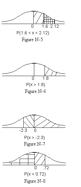
Figure N-5 asks us to determine the probability that a randomly selected value of x will be between 1.6 and 2.12. Both values are on the same side of the mean (the positive sice) and there is an overlap in the area under the curve for the two values. If we calculate the z values for both, find the probabilities, and subtract them the overlapped area will cancel and we will be left with the probability of a randomly selected value of x being between 1.6 and 2.12. z = (2.12 - 0)/1 = 2.12 and z = (1.6 - 0)/1 = 1.6. The associated probabilities (areas under the curve) from the z table are:0.9830 and 0.9452. Taking the difference 0.9830 - 0.9452 = 0.0378 which is the answer to the question.
Figure N-6 shows us a new question. Here we are asked to find the probability that a randomly drawn x will be greater than 1.8. We can use our normal technique, the x Score, to dermine the probability that x is between the mean (0) and 1.8. If you look that up in table A-2 you find that the probability is 0.4641. But that does not answer the question. We need to use the fact that the probability of a randomly selected value of x is above the mean (0) is 0.5. In other words half the values are above the mean and half are below. To determine the probability of a value of x being greater than 1.8 we must subtract 0.4641 from 0.5. The result and answer to the question is 0.5000 - 0.4641 = 0.0359.
Figure N-7 asks us to determine the probability that a randomly selected value of x is greater than -2.3. Greater than -2.3 includes all of the values above the mean. Using z = -2.3 we get a probability of 0.0107. To get the final answer we subtract 0.0107 from 1 the result is 0.9893, our final answer.
Figure N-8 twists the previous question around and asks us to determine the probability that a randomly selected value of x is below 0.72. We find the probability for a positive z of 0.72. The value is 0.7462. This is the answer to our question since it covers all of the area under the curve to the left (below) of 0.72.